Which Of The Following Is True While Applying The Excel Anova Tool?

ANOVA in Excel

Excel ANOVA(Table of Contents)

ANOVA in Excel
How to Find Anova Add-ins In excel?
How to Use ANOVA in Excel?

ANOVA in Excel

ANOVA (Analysis of Variance) in Excel is the single and two-factor method used to perform the null hypothesis test, which says if the test will be PASSED for Null Hypothesis if all the population values are exactly equal to each other. If any or at least one value is different from other values, then the null hypothesis will be FAILED. To perform ANOVA Test in Excel, from the Data menu tab, go to the Data Analysis option under the Analysis section and from there select ANOVA – Single Factor among other listed ANOVA Test. Select the input and output range as required. Once we get the output, we could conclude if we can consider or reject the data on the basis of the comparison of F and F-Critical values. If F < F-Critical, then we can consider the Null Hypothesis as PASSED, else FAILED.

ANOVA stands for Analysis of Variance. ANOVA in excel is a statistical method that is used to test the difference between two or more means.

Why ANOVA is used in excel?

In Microsoft excel, ANOVA- one-way analysis of variance is used to determine the factors of those mean are statistically significant or not, where mean square denotes the variation between the sample means, i.e. it simply test the null hypothesis.

How to Find Anova Add-ins In excel?

In excel, we can add the add-ins either by downloading from the internet or by purchasing the specific add-ins. Nowadays, we can find a huge number of add-ins on the internet which are available for download.

Excel comes with add-ins named Data analyzer, Solver etc… And few of the COM-add-ins which we can add in excel are Power Pivot, Power Query, Power View, etc…

Steps to add Anova add-ins In Excel

In excel, add-ins are always groped under the DATA menu by default, Excel does not have add-ins, and the data menu will appear.

In order to add add-ins in excel, follow the below steps.

In Excel, Go to the File menu.

Excel ANOVA Step 1

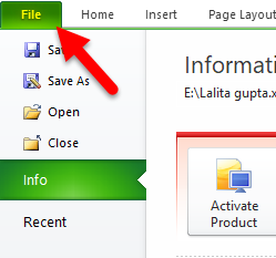
Choose Option where in the older version we can find the option called as "EXCEL OPTION".

Excel ANOVA Step 2

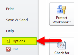
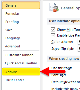
So that we will get the Excel options dialogue box window as shown below.

Excel ANOVA Step 3

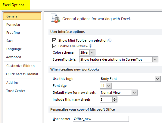
Now we can see add-ins; click on the add-ins.

Excel ANOVA Step 4

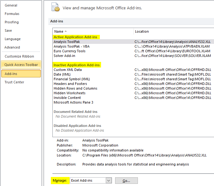
Once we click on the add-ins, we will get the window as shown below where it shows a list of add-ins; the first part shows the active Add-ins are installed which are being used in excel, and the second part shows that Inactive Add-ins that are no longer available in Excel.
At the bottom of the window, we can see the manage option where we can manage add-ins over here.

Excel ANOVA Step 5

Adding Excel- Add-ins

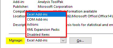
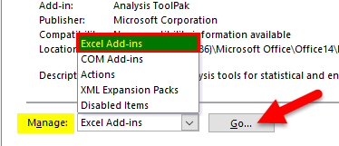
In excel, in the Manage option, we have add-ins option like Excel add-ins, COM add-ins, Action, XML expansion packs, Disabled Items.

Excel ANOVA Step 6

Let's see how to add excel-add in by following the below steps:

Click on the active add-in to add it in excel.
First, we will see how to activate Excel add-in in excel, which is shown in the first part.
Select the first add-ins Analysis ToolPack.

Excel ANOVA Step 6-1

And at the bottom, we can see the manager drop-down box in that select Excel-add-ins and then Click on the Go option.

Excel ANOVA Step 7

We will get the Add-Ins window as shown below.

Excel ANOVA Step 8

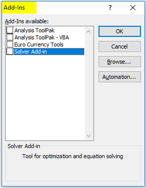
Now the analysis tool pack contains a set of add-ins that will allow us to choose it.
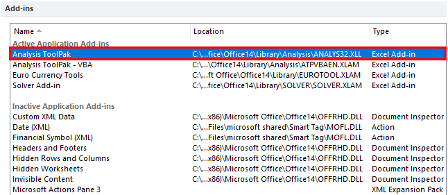
We can see that Analysis Tool Pack, Analysis Tool Pak-VBA, Euro Currency Tools, Solver Add-in.
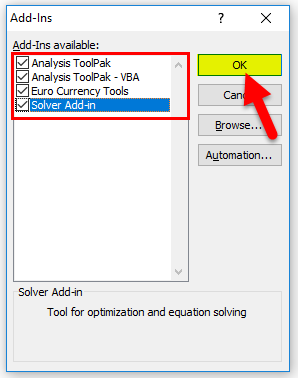
Check marks all add-ins and give OK so that selected add-ins will be get displayed in the data menu.

Excel ANOVA Step 9

After adding add-ins, we will have to check whether it's been added to the data menu or not.
Go to the Data menu, and at the right-hand side, we can see that add-ins are added, which is shown below.

Excel ANOVA Step 10

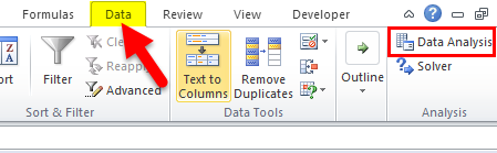
We can see in the data tab Data Analysis has been added under the analysis group, highlighted in Red color.

How to Use ANOVA in Excel?

ANOVA in excel is very simple and easy to use. Let's see the working of the excel ANOVA single factor built-in tool with some different Examples.

You can download this ANOVA Excel Template here – ANOVA Excel Template

Excel ANOVA – Example #1

In this example, we are going to see how to apply Excel ANOVA single factor by following the below example.

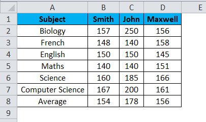
Consider the below example, which shows students marks scored on each subject.

ANOVA Example 1-1

Now we are going to check that student's marks are significantly different by using the ANOVA tool by following the below steps.

First, Go to the DATA menu and then click on the DATA ANALYSIS.

ANOVA Example 1-2

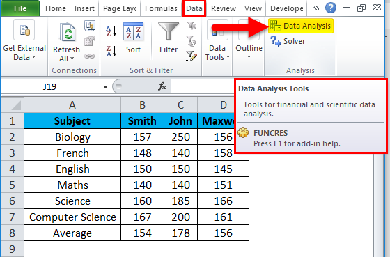
We will get the analysis dialogue box.
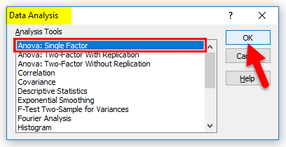
In the below screenshot, we can see the list of analysis tool where we can see the ANOVA- Single-factor tool.
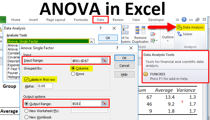
Click on the ANOVA: Single-factor tool and then click OK.

ANOVA Example 1-3

So that we will get the ANOVA: Single-factor dialogue box as shown in the below screenshot.

ANOVA Example 1-4

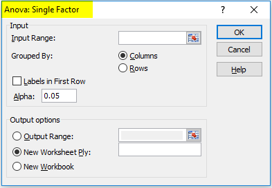
Now we can see the input range in the dialogue box.
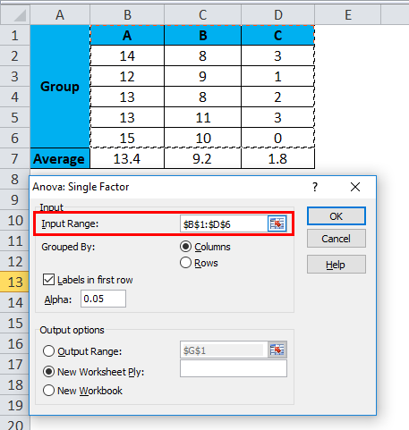
Click on the input range box to select the range $B$1:$D$7 as shown below.

ANOVA Example 1-5

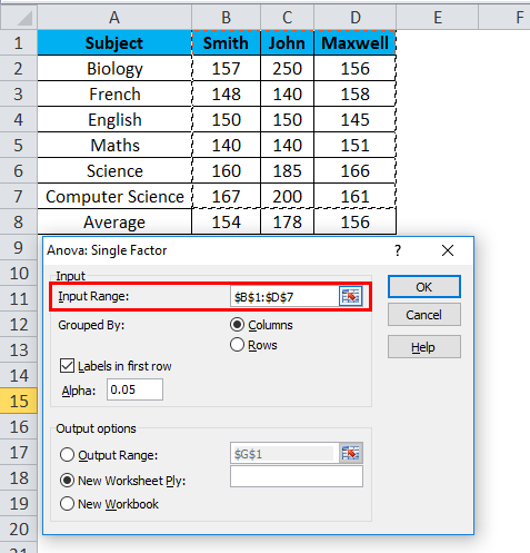
As we can see in the above screenshot, we have selected ranges along with the student name to get the exact output.
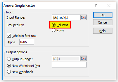
Now the input range has been selected, make sure thatColumn Checkbox is selected.

ANOVA Example 1-6

Next step, we want to select the output range where our output needs to be displayed.
Click on the output range box and select the output cell in the worksheet, which is shown below.

ANOVA Example 1-7

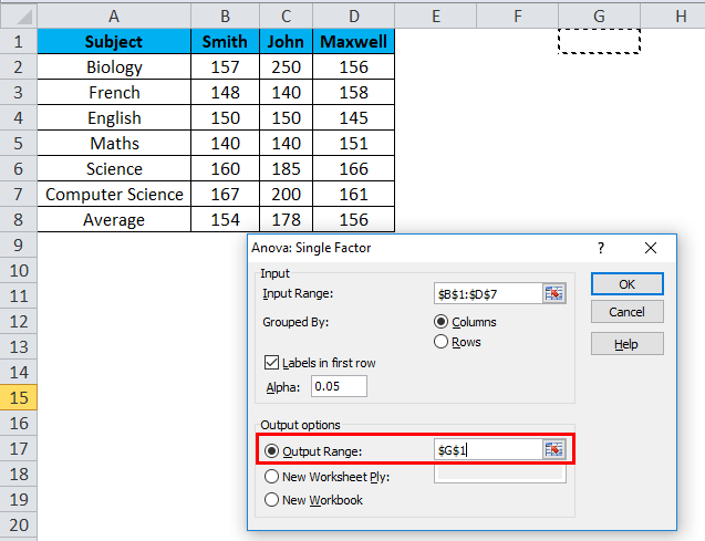
We have selected the output range cell as G1, where the output is going to be displayed.
Make sure thatLabels in the first-row Checkbox is selected, and then click on OK.

ANOVA Example 1-8

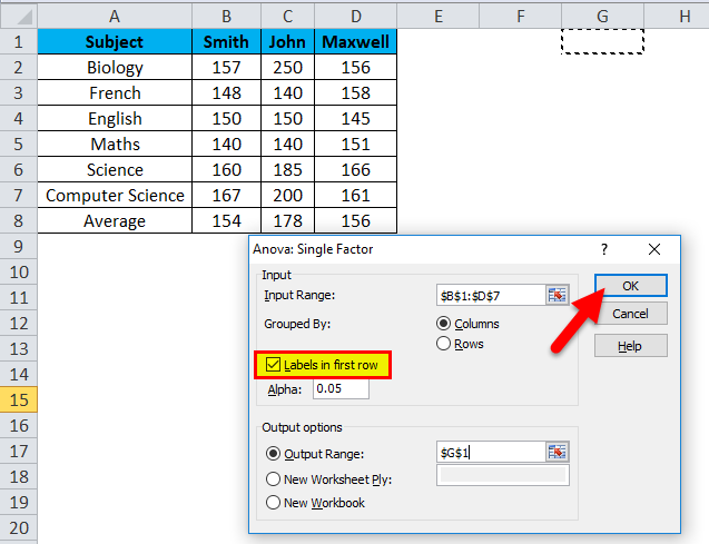
We will get the below output as follows.

A Example 1-9

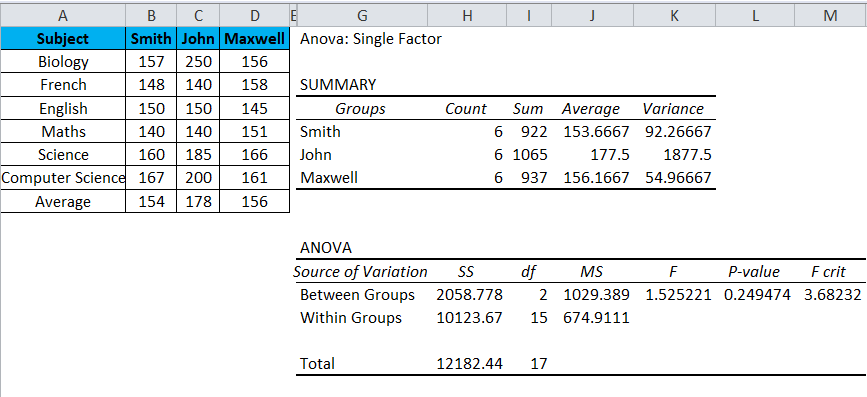
The above screenshot shows the summary part and Anova where the summary part contains the Group Name, No of Count, Sum, Average and Variance, and the Anova shows a list of summary where we need to check the F value and F Crit value.

F= Between Group /Within Group

F Statistic:The F statistic is nothing but values we get when we execute the ANOVA, which is used to determine the means between two populations significantly.

F values are always used along with the "P" value to check the results are significant, and it is enough to reject the null hypothesis.

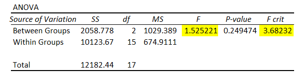
If we get the F value greater than the F crit value, then we can reject the null hypothesis, which means that something is significant, but in the above screenshot, we cannot reject the null hypothesis because F value is smaller than F critic and the student marks scored are not significant which is highlighted and shown in the below screenshot.

A Example 1-10

If we are running an excel ANOVA single factor, make sure that variance 1 is smaller than variance 2.

In the above screenshot, we can see that the first variance (92.266) is smaller than variance2 (1877.5).

Excel ANOVA – Example #2

In this example, we will see how to reject the null hypothesis by following the below steps.

A Example 2-1

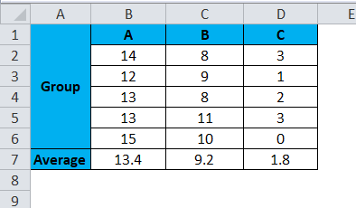
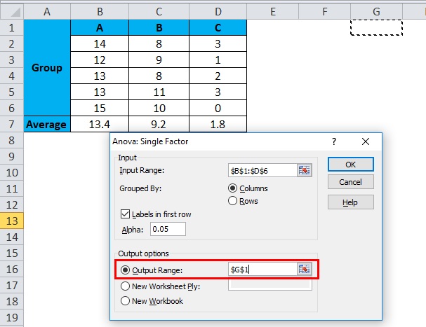
In the above screenshot, we can see the three groups A, B, C, and we are going to determine how these groups are significantly different by running the ANOVA test.

First, click on the DATA menu.
Click on the data analysis tab.
Choose Anova Single-factor from the Analysis dialogue box.
Now select the input range as shown below.

A Example 2-2

Next, select the output range as G1 to get the output.

A Example 2-3

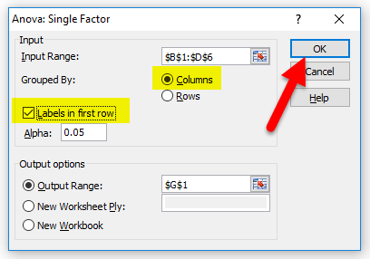
Make sure that Columns and Labels in the first-row Checkbox are selected, and then click on Ok.

A Example 2-4

We will get the below result as shown below.

A Example 2-5

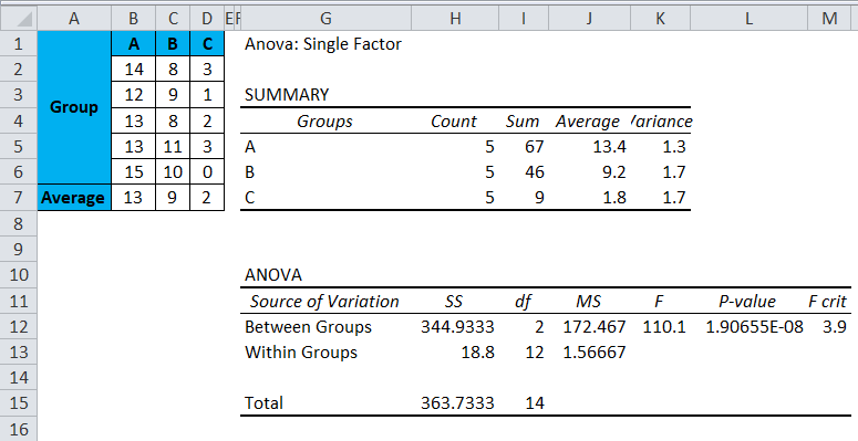
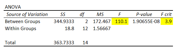
In the below screenshot, we can see that the F value is greater than the F crit value so that we can reject the null hypothesis, and we can say that at least one of the groups is significantly different.

A Example 2-6

Things to Remember

Excel ANOVA tool will work exactly if we have correct input or end up with wrong data.
Make sure that the first variance value is smaller than the second variance to get the exact F Value.